<?xml version="1.0" encoding="utf-8"?><feed xmlns="http://www.w3.org/2005/Atom" ><generator uri="https://jekyllrb.com/" version="3.10.0">Jekyll</generator><link href="https://gdubbs100.github.io/feed.xml" rel="self" type="application/atom+xml" /><link href="https://gdubbs100.github.io/" rel="alternate" type="text/html" /><updated>2026-03-08T00:16:25+00:00</updated><id>https://gdubbs100.github.io/feed.xml</id><title type="html">P(X = nonsense) &amp;lt; ε</title><subtitle>ML, RL and other topics I enjoy</subtitle><author><name>Grant Nicholas</name></author><entry><title type="html">Exploring the Cauchy distribution and electricity spot prices</title><link href="https://gdubbs100.github.io/2026/02/21/cauchy.html" rel="alternate" type="text/html" title="Exploring the Cauchy distribution and electricity spot prices" /><published>2026-02-21T00:00:00+00:00</published><updated>2026-02-21T00:00:00+00:00</updated><id>https://gdubbs100.github.io/2026/02/21/cauchy</id><content type="html" xml:base="https://gdubbs100.github.io/2026/02/21/cauchy.html"><![CDATA[<p>For a while now I’ve been fascinated by a probability distribution known as the Cauchy distribution. I first learnt about it through reading the books of Nicholas Nassim Taleb (The Black Swan, Antifragile) and later Benoit Mandelbrot (The (Mis)behaviour of Markets). Both of whom discuss the distribution in the context of financial risk.</p>

<p>The reason the Cauchy distribution is so fascinating is because it does not have a defined mean or variance. Essentially, if you sample from a Cauchy distribution, no matter how many samples you have, calculating the mean or variance of this distribution will not converge to a single value, contravening the central limit theorem. The variance, in fact, will diverge and is infinite. This is in stark contrast to distributions like the Gaussian, for which a rule of thumb is that 30 observations would give you a good estimate of its true parameters. Furthermore, the Cauchy distribution is no mathematical curio, it <a href="https://en.wikipedia.org/wiki/Cauchy_distribution#Occurrence_and_applications">occurs in the real world</a> in applications such as physics and finance.</p>

<p>With this in mind, I’m going to explore the properties of the Cauchy distribution and look at how it can be applied to Australian electricity spot-prices using a model developed by Powell <sup id="fnref:1" role="doc-noteref"><a href="#fn:1" class="footnote" rel="footnote">1</a></sup>.</p>

<h2 id="what-is-the-cauchy-distribution">What is the Cauchy distribution?</h2>
<p>As discussed above, the Cauchy distribution is a probability distribution with undefined mean and variance. The probability density function is defined as:</p>

\[f(x|x_{0}, \gamma) = \frac{1}{\pi}\frac{\gamma}{(x - x_{0})^2 + \gamma^2}\]

<p>Where $x_{0}$ is the location parameter, giving the centre of the distribution, and $\gamma$ is the scale parameter which is effectively the variance. Interestingly, with $x_{0} = 0, \lambda = 1$, the Cauchy distribution is identical to the student’s t-distribution with one degree of freedom (i.e. for two observations). This distribution can also be realised as the ratio of two independent Standard Gaussian distributions.</p>

<p>
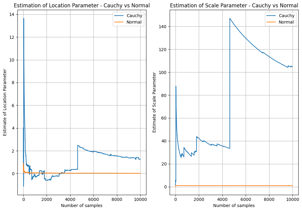
Below I’ve sampled $10,000$ observations from a $Cauchy(x_{0} = 0,\lambda = 1)$ and a $Normal(\mu = 0,\sigma^{2} = 1)$ distribution. I’ve estimated and plotted the mean and standard deviation on a rolling basis. The plot shows how the estimates of scale and location vary significantly for the Cauchy distribution.</p>

<p>On the left, after some initail volatility, the Cauchy location estimate appears to approach the true location (0), but suddenly jumps at around $x=5,000$ and fails to return to 0. In contrast, the Normal distribution quickly reaches almost exactly 0 and stays there as more samples are accumulated. On the right, the result is even worse - the estimate of the Scale (i.e. variance) gets larger as more samples are accumulated, while the estimate for the normal sits nicely at 1 - the true value.</p>

<p><img src="../../../images/20260221Cauchy/cauchy_behaviour.png" alt="Cauchy vs Normal Parameter Estimates" /></p>

<p>
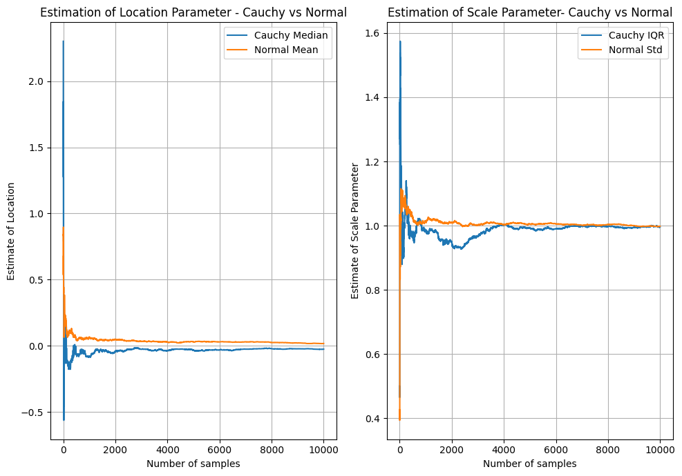
What this highlights, is that using the typical methods of estimating parameters like the location, that can work well for Gaussian, Exponential, Poisson and other distributions with finite mean/variance, does not work well for the Cauchy. This might come as a shock as the Maximum Likelihood Estimate (MLE) of the location parameters of these distributions is simply the arithmetic mean - probably the most widely used and understood statistic in existence! Naturally - there are a variety of ways of fitting the parameters of the Cauchy distribution. MLE is one way - noting that the arithmetic mean used above is <em>not</em> the MLE estimate of location for the Cauchy distribution. An even simpler way is to treat the location parameter as the median of the distribution and the scale as the inter-quartile range. Quantile estimates are less responsive to the extreme outliers that occur in the Cauchy distribution, hence they are more stable. The below plot compares these estimates for the same data and the same Gaussian mean/standard deviation estimates. You can see that both are much more stable and appear to reach the true value and remain stable.</p>

<p><img src="../../../images/20260221Cauchy/cauchy_median_iqr.png" alt="Cauchy median/iqr Parameter Estimates" /></p>

<h2 id="the-cauchy-distribution-and-electricity-spot-prices">The Cauchy Distribution and Electricity Spot Prices</h2>
<p>Observing this strange behaviour made me curious - it is all well and good observing this behaviour in the above contrived setup, but what about in the real world? In a sample of data taken from the real world, could you really see this kind of non-convergent behaviour?</p>

<p>I found one such instance in a paper by Kim and Powell <sup id="fnref:1:1" role="doc-noteref"><a href="#fn:1" class="footnote" rel="footnote">1</a></sup>, where they analyse electricity prices in the US and find that the Cauchy distribution is a good fit for modelling the error term of a median-reverting model of hourly spot prices. I decided to get some Australian data and see if I could replicate the model and view the Cauchy distribution in the wild.
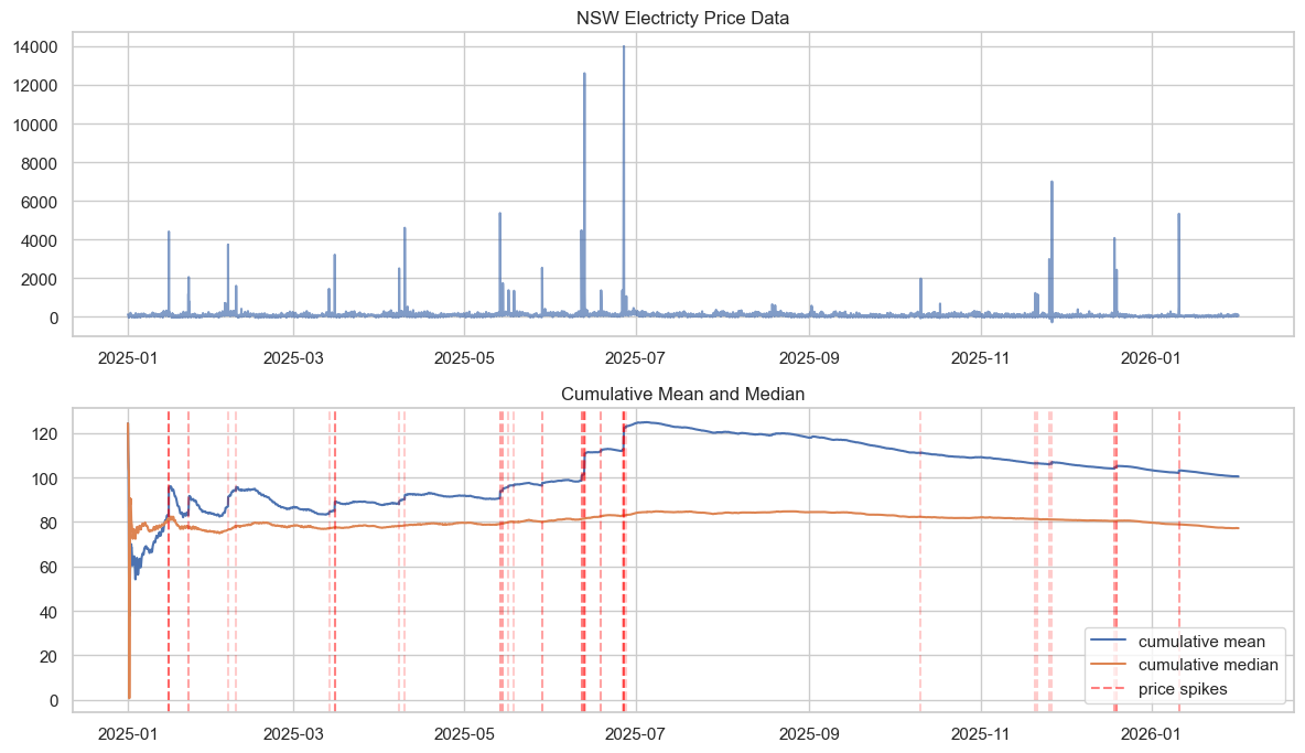
</p>

<p>Using the OpenElectricity API <sup id="fnref:2" role="doc-noteref"><a href="#fn:2" class="footnote" rel="footnote">2</a></sup> I was able to extract hourly electricty spot price data for NSW. Exactly the sort of data used in Kim and Powell’s paper. Plotting this price data below, we can see that the price behaviour is highly volatile with extreme spikes, and this affects the estimation of the mean. The mean estimate appears not to converge and be sensitive to sudden spikes, much like our simulated data above.</p>

<p>Over the course of the year, the trend electricity price may fluctuate due to seasonality, and this may mean we see a change in the mean - potentially resulting in non-convergence. But note, the types of changes we observe in the mean estimate are sudden and large, and they correlate with the extreme jumps in price (price spikes below are the 99.5th percentile price observations). This suggests that the reason for not converging is not due to seasonality or drift but rather the heavy tailed nature of the electricity prices. This is not to say there are no seasonal impacts on price - just that the instability in the mean estimate is not driven by them.</p>

<p><img src="../../../images/20260221Cauchy/nsw_price_behaviour.png" alt="NSW price behaviour" /></p>

<h3 id="a-median-reversion-model-of-electricity-prices">A Median Reversion Model of Electricity Prices</h3>

<p>Powell and Kim develop a model of hourly electricity spot prices which assumes that prices revert towards the median <sup id="fnref:1:2" role="doc-noteref"><a href="#fn:1" class="footnote" rel="footnote">1</a></sup>. Their objective is to accurately model the tails of the price distribution to enable effective trading in the energy market. Their model follows the below equation:</p>

\[p_{t+1} = p_{t} + (1 - \kappa) (p_{t} - \mu_{t}) \hat{\epsilon}_{t}\]

<p>Where:</p>
<ul>
  <li>$\kappa = (1 - \bar{\mu}_{Y})$</li>
  <li>$\bar{\mu}_{Y} = \text{median}(Y_{t})$;</li>
  <li>$Y_{t}$ is the residual term;</li>
  <li>$\mu_{t}$ is a trailing monthly price median which accounts for seasonal variation in prices;</li>
  <li>$\hat{\epsilon}_{t}$ is the error estimate applied multiplicatively to the median reversion term.</li>
</ul>

<p>Essentially, this model assumes that there is large uncertainty when the current price has deviated from the rolling monthly median. Naturally, the use of the median is driven by their analysis of the electricity prices where they observe a non-convergent mean.</p>

<p>It is worth looking at the residual $Y_{t}$ and error term $ \hat{\epsilon}_{t} $.</p>

\[Y_{t} = \frac{(p_{t} - p_{t - 1})}{(\mu_{t - 1} - p_{t - 1})}\]

<p>Which is the ratio of the change in price to the deviation of price from the trailing median. Note that for the next step ahead prediction, $1 - \kappa = 1 - (1 - \mu_{Y}) = \mu_{Y}$ which implies that the strength of the median reversion is governed by the median value of the residual. That is, the median ratio of price changes to the difference between the price to the median monthly price is an estimate of how much pull there is back to the median price. If we have small price changes relative to that prices distance from the median, then there is only a small pull back to the median, in contrast if the changes are large, then there is a strong pull back to the centre.</p>

<p>The error term is given by:</p>

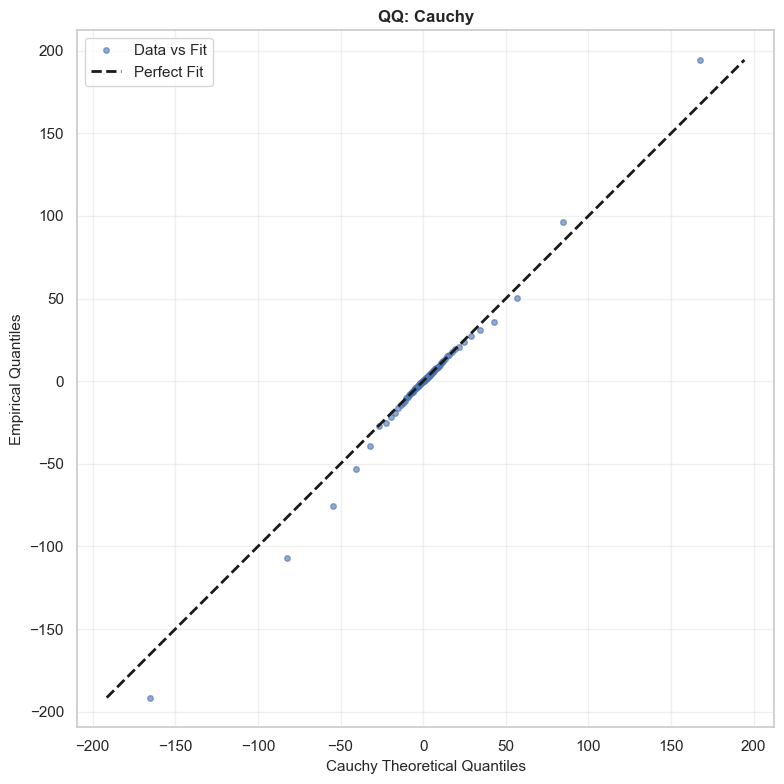
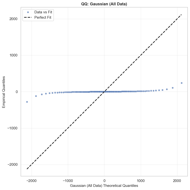
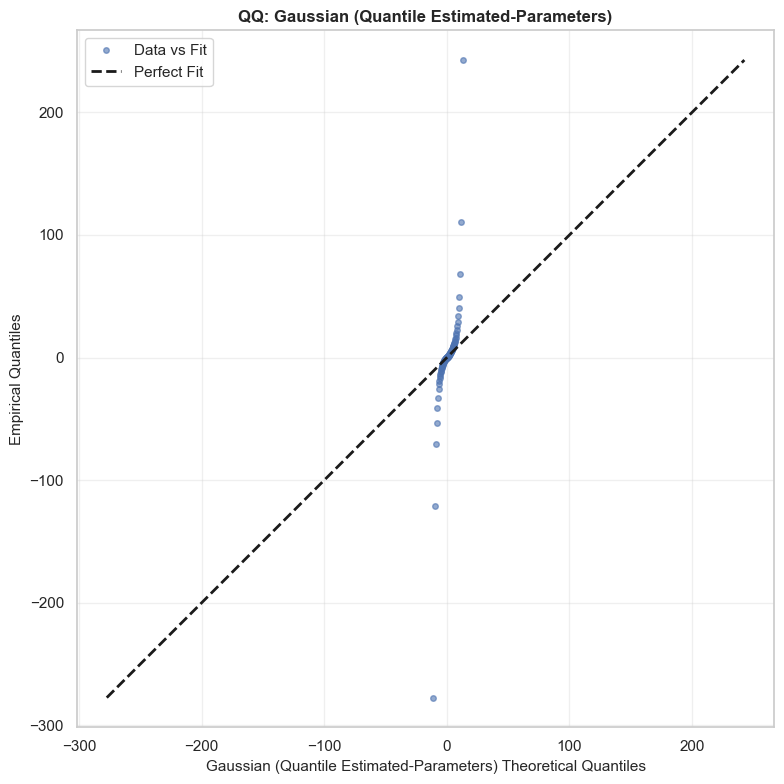
\[\hat{\epsilon}_{t} = \frac{Y_{t}}{\mu_{Y}}\]

<p>This is the term that Kim and Powell suggest is governed by a Cauchy distribution. In their paper, they estimate the tail parameter $\alpha$ and find that it is close to 1, implying infinite variance. <sup id="fnref:1:3" role="doc-noteref"><a href="#fn:1" class="footnote" rel="footnote">1</a></sup> I’ve simply done a comparison here against a QQ-plot looking at the actual data vs a Cauchy distribution with $x_0 = 1$ and $\gamma \approx 5.23$. I’ve also estimated a Gaussian with $\mu \approx -3.5$ and $\sigma \approx 911$ (naively, without removing outliers), and another Gaussian using the same parameters as the Cauchy distribution - i.e. with Quantile Estimated Parameters (QEP). You can see clearly that the Cauchy distribution fits significantly better than either of the Gaussians,with each of these significantly over or under estimating the frequency for the tails. The Cauchy distribution is not perfect however, and appears to have more extreme tails than the actual data. Note, the analysis hereon is applied to a test set (Jan to mid Feb 2026) which was not used to fit the distributions or model. The training set comprised of NSW hourly spot price data for all of 2025.</p>

<div style="display: flex; justify-content: space-between; gap: 10px;">
  <figure style="width: 30%; text-align: center;">
    <img src="/images/20260221Cauchy/qq_cauchy_test.png" alt="Cauchy QQ Plot" />
    <figcaption><b>Cauchy distribution</b></figcaption>
  </figure>
  
  <figure style="width: 30%; text-align: center;">
    <img src="/images/20260221Cauchy/qq_normal_test_all.png" alt="Gaussian QQ Plot" />
    <figcaption><b>All-data Normal distribution</b></figcaption>
  </figure>

  <figure style="width: 30%; text-align: center;">
    <img src="/images/20260221Cauchy/qq_normal_test_qep.png" alt="QEP Gaussian QQ Plot" />
    <figcaption><b>QEP Normal distribution</b></figcaption>
  </figure>
</div>

<p>Quantile distributions of $Y$ show a good match as well (this is how Powell and Kim present their model fit before concluding the paper). You can see, the Cauchy quantiles match nicely with the actual distribution, while the naive Gaussian distribution are far from the mark around the tails. Essentially, while the variance is clearly large - the spread of prices between the 90th and 10th quantiles is over $2,000 for the naive estimate - the Gaussian distributions fail to account for the fact that there are massive <em>rare</em> events. They just assume that 80% of prices will be somewhere between +/- $1,000. This is not very specific and does not reflect the true distribution of prices.</p>

\[\small
\begin{array}{|l|r|r|r||r|r|r|r|}
\hline
\text{Model} &amp; \text{0.1} &amp; \text{0.2} &amp; \text{0.3} &amp; \text{0.4} &amp; \text{0.5} &amp; \text{0.6} &amp; \text{0.7} &amp; \text{0.8} &amp; \text{0.9} \\ \hline
\text{Actual} &amp; -15.998 &amp; -6.245 &amp; -2.562 &amp; -0.503 &amp; 1.016 &amp; 2.711 &amp; 4.807 &amp; 8.089 &amp; 17.546 \\
\text{Cauchy} &amp; -15.108 &amp; -6.204 &amp; -2.802 &amp; -0.701 &amp; 1.000 &amp; 2.701 &amp; 4.802 &amp; 8.204 &amp; 17.108 \\
\text{Gaussian (QE-P)} &amp; -5.707 &amp; -3.405 &amp; -1.745 &amp; -0.326 &amp; 1.000 &amp; 2.326 &amp; 3.745 &amp; 5.405 &amp; 7.707 \\ 
\text{Gaussian (All Data)} &amp; -1171.762 &amp; -770.723 &amp; -481.545 &amp; -234.454 &amp; -3.503 &amp; 227.447 &amp; 474.539 &amp; 763.716 &amp; 1164.755 \\\hline
\end{array}\]

<p>We can see this better when we look at actual prices. Below we plot the prices and predictions on the first week of test data. The distribution around the prices varies significantly between the error terms. As we saw in the quantile plot above, the all-data Gaussian distribution has unrealistically large tails. Almost every observation occurs well within the IQR of the Gaussian distribution - which should truly only have 50% of the observations. In contrast, the QEP Gaussian has tails that are two narrow. When prices shift up or down rapidly, prices will often sit ouside of the 95% CI entirely. The behaviour of the Cauchy distribution is much nicer - the IQR is appropriately narrow, and captures many observations. The 95% CI is much wider, and often captures prices when they grow rapidly.</p>

<div style="justify-content: space-between; gap: 10px;">
  <figure style="width: 100%; text-align: center;">
    <img src="/images/20260221Cauchy/all_data_gaussian_test.png" alt="Cauchy Error Price Model" />
    <figcaption><b>Gaussian (all-data) Error on a typical week</b></figcaption>
  </figure>
  <figure style="width: 100%; text-align: center;">
    <img src="/images/20260221Cauchy/qep_gaussian_test.png" alt="Gaussian (filtered data) Error Price Model" />
    <figcaption><b>Gaussian (Quantile Estimated Parameters) Error on a typical week</b></figcaption>
  </figure>
  
  <figure style="width: 100%; text-align: center;">
    <img src="/images/20260221Cauchy/cauchy_test.png" alt="Cauchy Error Price Model" />
    <figcaption><b>Cauchy Error on a typical week</b></figcaption>
  </figure>


</div>

<p>
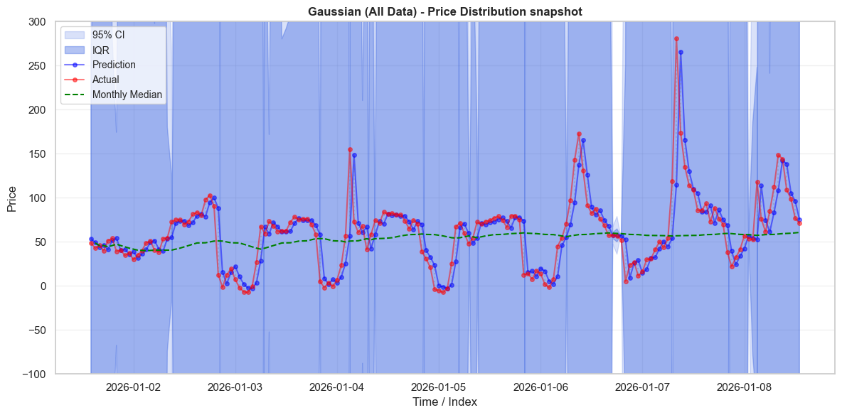
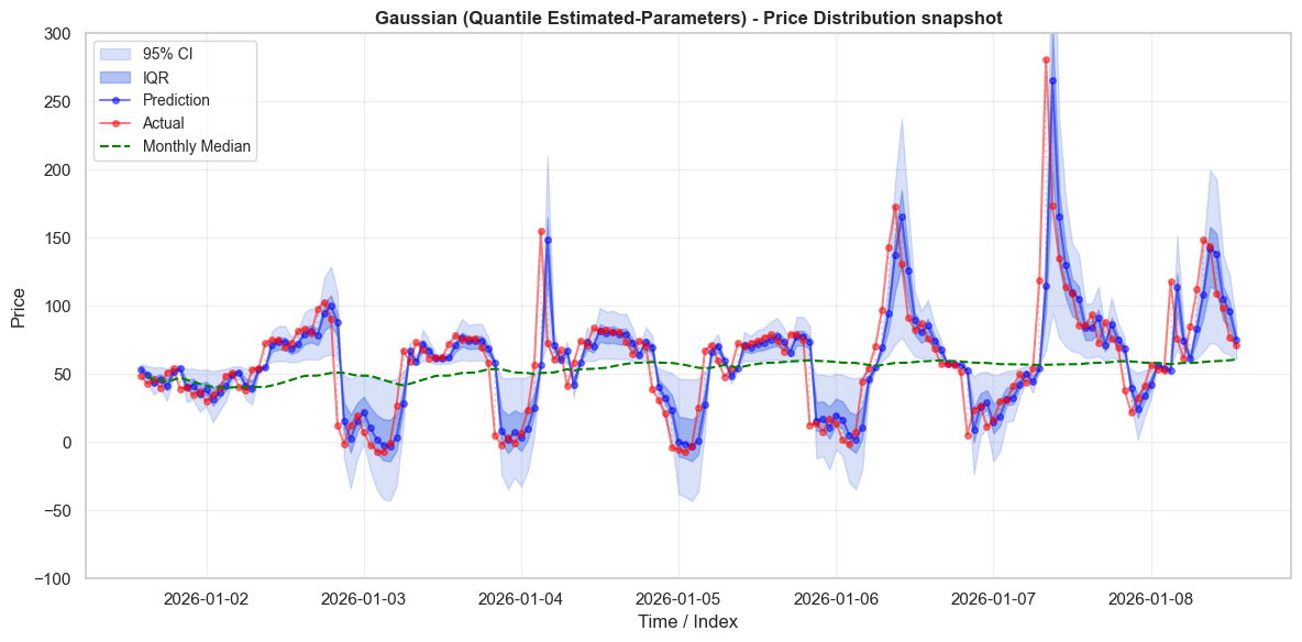
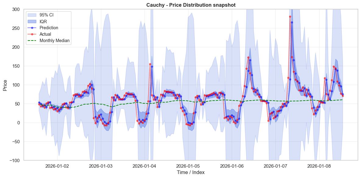
A third demonstration that the Cauchy distribution is the best of the three distributions considered is provided in the below table. The Cauchy distribution captures exactly 50% of price observations in its IQR, and just shy of 95% within the 95% CI. In contrast, the naive Gaussian distribution thinks that almost <em>everything</em> should fall within the IQR. It over states the probability of events occurring because it is highly responsive to the outliers in the data. While this distribution might assign every observed price a high probability, it doesn’t assign it an <em>accurate</em> probability, which is a problem if you want it to guide decision making. As anticipated, the QEP Gaussian under-estimates probabilities, with under 40% falling within its IQR and only 70% within its 95% CI.</p>

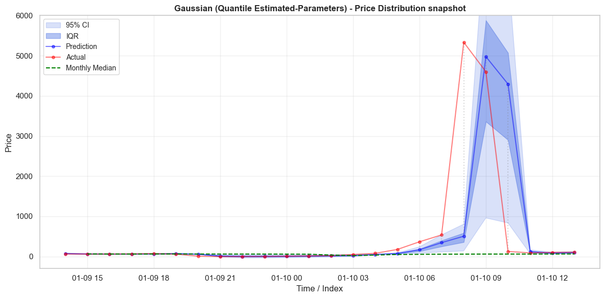
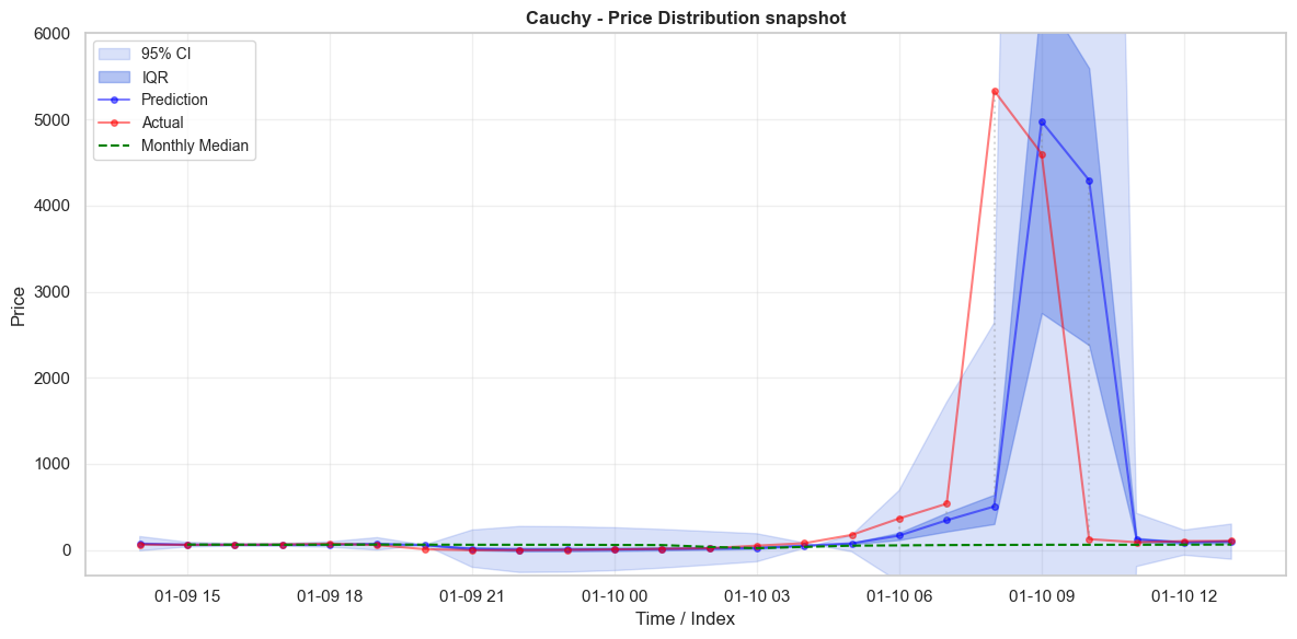
\[\small
\begin{array}{|l|c|c|c|c|}
\hline
\text{Distribution} &amp; \text{Test in IQR} &amp; \text{Train in IQR} &amp; \text{Test in 95 CI} &amp; \text{Train in 95 CI} \\ \hline
\text{Cauchy} &amp; 0.500 &amp; 0.499 &amp; 0.938 &amp; 0.938 \\ \hline
\text{Gaussian (QEP)} &amp; 0.388 &amp; 0.388 &amp; 0.702 &amp; 0.683 \\ \hline
\text{Gaussian (All Data)} &amp; 0.989 &amp; 0.991 &amp; 0.993 &amp; 0.996 \\ \hline
\end{array}\]

<p>Before finishing, I did want to analyse a price spike that occurs in the test data. Its interesting to see that despite its fatter tails, the Cauchy distribution can still miss outliers by potentially a large amount. It does do significantly better than the QEP Gaussian distribution which fails to include the whole trajectory leading up to the spike in its 95% CI. While the Cauchy distribution seems significantly better as a decision making guide, there is still the possibility of making very large mistakes.</p>

<div style="justify-content: space-between; gap: 10px;">
  <figure style="width: 100%; text-align: center;">
    <img src="/images/20260221Cauchy/qep_gaussian_test_spike.png" alt="Gaussian Error Price Model" />
    <figcaption><b>Gaussian (Quantile-Estimated Parameters) Error on price spike</b></figcaption>
  </figure>
  
  <figure style="width: 100%; text-align: center;">
    <img src="/images/20260221Cauchy/cauchy_test_spike.png" alt="Cauchy Error Price Model" />
    <figcaption><b>Cauchy Error on price spike</b></figcaption>
  </figure>
</div>

<h2 id="conclusion">Conclusion</h2>
<p>So we have seen that despite their unusual properties of not having undefined means and variances, the Cauchy distribution does occur in real world circumstances and can be applied in modelling them. One thing I’d be interested in learning more about is how to use a model such as the one implemented above. As it was designed for energy trading, I think it would be interesting to understand what strategies it could be used for. The first thing that comes to mind is for buying low / selling high with a probabilitistic forecast of future prices. But I do note - while the Cauchy model appears to have generally accurate predictions, it still seems capable of missing large price spikes. Furthermore, the model described above relies only on past prices - which likely have limited predictive power. Incorporating other features such as weather could be another interesting area to explore further.</p>

<h2 id="references">References</h2>
<div class="footnotes" role="doc-endnotes">
  <ol>
    <li id="fn:1" role="doc-endnote">
      <p>Kim, J. H., &amp; Powell, W. B. (2011). An hour-ahead prediction model for heavy-tailed spot prices. <em>Energy Economics</em>, 33(6), 1252-1266. https://doi.org/10.1016/j.eneco.2011.06.007 <a href="#fnref:1" class="reversefootnote" role="doc-backlink">&#8617;</a> <a href="#fnref:1:1" class="reversefootnote" role="doc-backlink">&#8617;<sup>2</sup></a> <a href="#fnref:1:2" class="reversefootnote" role="doc-backlink">&#8617;<sup>3</sup></a> <a href="#fnref:1:3" class="reversefootnote" role="doc-backlink">&#8617;<sup>4</sup></a></p>
    </li>
    <li id="fn:2" role="doc-endnote">
      <p><strong>Open Electricity.</strong> (2024). <em>OpenElectricity API and Platform</em>. The Superpower Institute. Available at: <a href="https://openelectricity.org.au">https://openelectricity.org.au</a> (Accessed: 24 February 2025). <a href="#fnref:2" class="reversefootnote" role="doc-backlink">&#8617;</a></p>
    </li>
  </ol>
</div>]]></content><author><name>Grant Nicholas</name></author><category term="Other" /><summary type="html"><![CDATA[For a while now I’ve been fascinated by a probability distribution known as the Cauchy distribution. I first learnt about it through reading the books of Nicholas Nassim Taleb (The Black Swan, Antifragile) and later Benoit Mandelbrot (The (Mis)behaviour of Markets). Both of whom discuss the distribution in the context of financial risk.]]></summary></entry><entry><title type="html">Model Predictive Control with black-box dynamics models</title><link href="https://gdubbs100.github.io/2026/01/24/MPC.html" rel="alternate" type="text/html" title="Model Predictive Control with black-box dynamics models" /><published>2026-01-24T00:00:00+00:00</published><updated>2026-01-24T00:00:00+00:00</updated><id>https://gdubbs100.github.io/2026/01/24/MPC</id><content type="html" xml:base="https://gdubbs100.github.io/2026/01/24/MPC.html"><![CDATA[<h4 id="tldr">TLDR</h4>
<ul>
  <li>Model Predictive Control algorithms are algorithms that enables us to exploit knowledge of the world to solve sequential decision problems rapidly.</li>
  <li>These algorithms can be applied without knowledge of the environment dynamics, using methods such as Random Shooting, the Cross-Entropy-Method, and Model Predictive Path Integral.</li>
  <li>Gradient Based Methods are also an option if you have a differentiable dynamics model or environment.</li>
  <li>I’ve developed some implementations in this <a href="https://github.com/gdubbs100/mpc_experiment/tree/main">repository</a> and exhibit their performance on a simple environment.</li>
</ul>

<h2 id="why-model-predictive-control">Why Model Predictive Control?</h2>

<p>If you’ve ever played around with Reinforcement Learning (RL), no doubt you have experienced frustrations with long training times, silent bugs and brittle algorithms that improve up until they suddenly don’t. It’s a <a href="https://spinningup.openai.com/en/latest/spinningup/spinningup.html">common experience</a> for RL enthusiasts and one that has grated across my nerves as I’ve tinkered with RL. A key frustration of mine is how long it takes for deep RL algorithms to learn even the simple environments provided in <a href="https://gymnasium.farama.org/">Gymnasium</a>.</p>

<p>Consequently, I was interested to see Yann LeCunn’s oft quoted statement: <a href="https://drive.google.com/file/d/1BU5bV3X5w65DwSMapKcsr0ZvrMRU_Nbi/view"> “Abandon Reinforcement Learning in favour of Model Predictive Control”</a>. Model Predictive Control (MPC) uses a dynamics model and reward function to determine optimal actions. Using this approach you can achieve good performance on tasks really quickly (even within a single episode), the key challenge and caveat being - you need a reasonable dynamics model. This may be available in domains such as physics where the world is well understood and predictable, but more challenging in general applications.</p>

<p>Hence, I decided to explore MPC and how to implement it. A key challenge I found - and a motivation for writing this article - was that many resources on MPC were either too basic or too technical. MPC is a branch of optimal control and often assumes an engineering background with significant knowledge of physics or other branches of science. Many expositions of the topic would dive into complex case studies where the specifics of the dynamics models were discussed in great detail. Reading these without the requisite background made it hard to understand what MPC actually did. In contrast, many other introductions were absurdly simple - they would describe the process at a high level, but then crucial details required for implementation were absent.</p>

<p>Eventually, after more digging, and (to be perfectly honest) asking ChatGPT, I was able to understand and implement some MPC algorithms which were application agnostic. Given the effort this took, I thought it would be a worthwhile task to write an article on these methods which avoids getting bogged down in the minutae of dynamics models and applications, but still provides the key details needed for implementation. I’ve also provided a <a href="https://github.com/gdubbs100/mpc_experiment/tree/main">repository</a> with the implementations and a toy environment.</p>

<h2 id="so-what-is-mpc">So what is MPC?</h2>
<p>MPC is a relatively simple algorithm used to solve sequential decision problems. MPC involves selecting actions that will maximise a reward (or minimise a cost) in an environment. These rewards are calculated using a forward looking dynamics model which simulates the impact of the selected actions on the environment. The typical approach is to generate actions for k-steps into the future, run these actions through the dynamics model, and then evaluate the total reward of those actions. You run several of these simulations and pick the first action from the best trajectory (i.e. the trajectory that achieves the best reward or lowest cost). You repeat this everytime you need to make a decision, thus enabling you to choose actions which should maximise the reward over a forward window based on your knowledge of the environment.</p>

\[\begin{array}{l}
\hline
\textbf{Algorithm: } \text{Model Predictive Control (MPC) Framework} \\
\hline
\textbf{Input: } \text{State } x_t, \text{ Horizon } k, \text{ Samples } N, \text{ Model } f_\theta, \text{ Reward } R, \text{ Terminal Reward } \phi \\
\textbf{Output: } \text{Optimal first action } u_t^* \\
\hline
1: \text{Generate } N \text{ candidate action sequences: } \{ \mathbf{u}^{(i)}_{0:k-1} \}_{i=1}^N \\
2: \textbf{for } \text{each sequence } i = 1 \dots N \textbf{ do} \\
3: \quad \text{Roll out trajectory: } \hat{x}_{j+1} = f_\theta(\hat{x}_j, u_j) \text{ for } j = 0 \dots k-1 \\
4: \quad \text{Calculate reward: } J^{(i)} = \phi(\hat{x}_{k-1}) + \sum_{j=0}^{k-1} R(\hat{x}_j, u_j) \\
5: \textbf{end for} \\
6: \text{Select best sequence: } i^* = \arg\max_i J^{(i)} \\
7: \textbf{return } u_t^* = \mathbf{u}^{(i^*)}_{0} \\
\hline
\end{array}\]

<p>So far so good - but we need to think a bit more before we can actually implement this algorithm:</p>

<ol>
  <li>How do you generate sequences of actions?</li>
  <li>How do you ensure that the sequences you generate are any good??</li>
  <li>How do you get this dynamics model $f_\theta$?</li>
  <li>What is the reward model $R$?</li>
</ol>

<p>The MPC algorithms I will discuss below offer different ways to answer questions 1 and 2 above. They are designed to generate a set of actions, and then use the outputs of the dynamics and reward functions to optimise these actions. That is, they find the actions that maximise the reward (or minimise the cost) over the next k-steps in the future.</p>

<p>Before proceeding, on points 3, 4, while the dynamics model and rewards model are essential to the implementation of MPC, they are also inputs to the MPC algorithm and their actual forms will depend on the problem being solved. For this article, I will ignore them. Suffice to say the dynamics model is given - possibly learnt - while the reward function will often look something like this:</p>

\[R(x_{t}, u_{t})=-(x_{t}Px_{t}^{T} + u_{t}Qu_{t}^{T})\]

<p>where we apply a negative sign because we’re talking about reward rather than cost, $x_{t}$, $u_{t}$ are the states and actions at time $t$, $P$ is a cost matrix for states (for example a penalty based on distance from a target state) and $Q$ is a cost matrix for actions (i.e. we might want to incentivise smaller actions). In any case, as the objective of my article is to avoid getting bogged down in the specifics of the dynamics models and applications, I’ll assume that these components are given.</p>

<h2 id="implementing-mpc">Implementing MPC</h2>
<h3 id="1-random-shooting">1. Random Shooting</h3>
<p>The simplest approach is to generate actions by random sampling. We select a rollout length of $k$, a number of rollouts $n$, and then randomly sample $k \times n$ actions (e.g. from a standard normal distribution) and pass each of these through our dynamics model. Take the action trajectory which achieved the best reward and take the first action from that trajectory to be applied in the environment.</p>

\[\begin{array}{l}
\hline
\textbf{Algorithm: } \text{Random Shooting} \\
\hline
\textbf{Input: } \text{State } x_t, \text{ Horizon } k, \text{ Samples } N, \text{ Model } f_\theta, \text{ Reward } R, \text{ Terminal Reward } \phi \\
\textbf{Output: } \text{First action } u_t^* \\
\hline
1: \text{Sample } N \text{ sequences from distribution: } \mathbf{u}^{(i)}_{0:k-1} \sim \mathcal{N}(\mathbf{0}, \mathbf{I}) \\
2: \textbf{for } \text{each sequence } i = 1 \dots N \textbf{ do} \\
3: \quad \text{Roll out trajectory: } \hat{x}_{j+1} = f_\theta(\hat{x}_j, u_j) \\
4: \quad \text{Calculate reward: } J^{(i)} = \phi(\hat{x}_{k-1}) + \sum_{j=0}^{k-1} R(\hat{x}_j, u_j) \\
5: \textbf{end for} \\
6: \text{Select best sequence: } i^* = \arg\max_i J^{(i)} \\
7: \textbf{return } u_t^* = \mathbf{u}^{(i^*)}_{0} \\
\hline
\end{array}\]

<p>Random shooting is simple to implement and quick to run, however, you might wonder how well you can select the correct actions simply by random sampling. In addition, there is no learning or refinement of actions. In that respect, random shooting is inefficient in generating good actions as the only rollout that determines your reward is the one you select - but you ignore all the other rollouts. This is suboptimal because those rollouts contain valuable information about how selected actions can affect rewards.</p>

<h3 id="2-the-cross-entropy-method-cem">2. The Cross-Entropy-Method (CEM)</h3>
<p>CEM is a genetic algorithm or population-based method, which randomly samples actions and then refines those actions by aggregating the top-m or top-$\alpha$ percentile reward-achieving-trajectories <sup id="fnref:1" role="doc-noteref"><a href="#fn:1" class="footnote" rel="footnote">1</a></sup>. The algorithm works much like the random-shooting algorithm with the addition of the refinement process.</p>

<p>As a concrete example, assume we sample actions from a standard normal distribution: $ a_{t} \sim N(0, 1) $. We then run trajectories through the dynamics model and rank them by achieved rewards. We select the $m$ best, or use a percentile cutoff, to create a subset of trajectories referred to as “elites”. Using only these elites we recalculate the entries of the mean and standard deviation of the sampling distribution from the corresponding vector position of the elites. That is, we maintain and update a normal distribution for each step of the rollout. After a $I$ learning iterations, we can sample an action from the first distribution or just take the mean.</p>

\[\begin{array}{l}
\hline
\textbf{Algorithm: } \text{Cross-Entropy Method (CEM)} \\
\hline
\textbf{Input: } \text{State } x_t, \text{ Horizon } k, \text{ Samples } N, \text{ Elites } m, \text{ Iterations } I, \text{ Model } f_\theta, \dots \\
\textbf{Initialize: } \mu_{j} = \mathbf{0}, \sigma_{j} = \mathbf{I} \text{ for } j = 0 \dots k-1 \\
\hline
1: \textbf{for } \text{iteration } 1 \dots I \textbf{ do} \\
2: \quad \text{Sample } N \text{ sequences: } \mathbf{u}^{(i)}_{0:k-1} \sim \mathcal{N}(\mu_{0:k-1}, \sigma_{0:k-1}) \\
3: \quad \textbf{for } \text{each sequence } i = 1 \dots N \textbf{ do} \\
4: \quad \quad \text{Roll out trajectory: } \hat{x}_{j+1} = f_\theta(\hat{x}_j, u_j) \\
5: \quad \quad \text{Calculate reward: } J^{(i)} = \phi(\hat{x}_{k-1}) + \sum_{j=0}^{k-1} R(\hat{x}_j, u_j) \\
6: \quad \textbf{end for} \\
7: \quad \text{Select set of } m \text{ elite sequences with highest } J^{(i)} \\
8: \quad \text{Update } \mu_j = \text{mean}(\text{elites}_j), \sigma_j = \text{std}(\text{elites}_j) \text{ for } j = 0 \dots k-1 \\
9: \textbf{end for} \\
10: \textbf{return } u_t^* = \mu_0 \\
\hline
\end{array}\]

<p>One benefit of the CEM algorithm is that it is completely agnostic of the structure of the problem to which it is applied. It is a general purpose optimisation algorithm which can be applied in many domains <sup id="fnref:1:1" role="doc-noteref"><a href="#fn:1" class="footnote" rel="footnote">1</a></sup>. However, this is also a weakness as it means its sampling and updates of actions do not learn from the structure of the environment - this is a missed opportunity and can lead to slower optimisation. CEM reportedly also struggles with high dimensional action spaces <sup id="fnref:2" role="doc-noteref"><a href="#fn:2" class="footnote" rel="footnote">2</a></sup>. Despite this, it is a flexible algorithm and is relatively simple to implement.</p>

<h3 id="3-model-predictive-path-integral-mppi">3. Model Predictive Path Integral (MPPI)</h3>
<p>MPPI is another population based method which is based around the concept of an ‘optimal information theoretic control law’ <sup id="fnref:3" role="doc-noteref"><a href="#fn:3" class="footnote" rel="footnote">3</a></sup> <sup id="fnref:4" role="doc-noteref"><a href="#fn:4" class="footnote" rel="footnote">4</a></sup>. Essentially, MPPI learns a distribution of over actions by minimising the <a href="https://en.wikipedia.org/wiki/Kullback%E2%80%93Leibler_divergence">Kullback-Leibler Divergence</a> between the action sampling distribution and the optimal control distribution given by <sup id="fnref:5" role="doc-noteref"><a href="#fn:5" class="footnote" rel="footnote">5</a></sup>:</p>

\[\frac{1}{Z}\exp({-\frac{1}{\lambda}J})\]

<p>Which is the weighted expected average reward, normalized by $Z$, with a temperature parameter $\lambda$ - larger values of which result in a more uniform distribution. This distribution is a boltzmann distribution that assigns higher probabilities to trajectories with lower costs.</p>

<p>The MPPI algorithm assumes that an action isn’t directly applied in the environment. Rather there is a stochastic relationship between the action intended and the action that actually ends up being applied in the system, given by $v_{t} \sim N(u_{t}, \Sigma)$. The algorithm starts by sampling noise $\epsilon_{t} \sim N(0, 1)$ and combining this with a base set of actions $v_{t} = u_{t} + \epsilon_{t}$ and collecting rewards via dynamics model simulation. Once collecting the rewards, MPPI updates the actions $u_{t}$ using a weighted average of the rewards:</p>

\[u_{t}^{(i)} = u_{t}^{(i-1)} + \sum^{N}_{n=1}{w}\epsilon_{n}^{(i-1)}\]

<p>Where the weighting is given by <sup id="fnref:3:1" role="doc-noteref"><a href="#fn:3" class="footnote" rel="footnote">3</a></sup>:</p>

\[w = \frac{1}{Z}\exp({-\frac{1}{\lambda}(J^{(k)} - \text{max}(J))})\]

<p>This weighting is just the optimal distribution discussed above. The subtraction of the maximum value of $J$ (max because we’re using reward rather than cost) helps stabilise the weighting.</p>

\[\begin{array}{l}
\hline
\textbf{Algorithm: } \text{Model Predictive Path Integral (MPPI)} \\
\hline
\textbf{Input: } \text{State } x_t, \text{ Horizon } k, \text{ Samples } N, \text{ Temp } \lambda, \text{ Noise } \Sigma, \text{ Model } f_\theta, \dots \\
\textbf{Initialize: } \text{Mean action sequence } \mathbf{u}_{0:k-1} \\
\hline
1: \textbf{for } \text{iteration }1 \dots I \textbf{ do} \\
2: \quad \text{Sample } N \text{ noise sequences: } \epsilon^{(n)}_{0:k-1} \sim \mathcal{N}(0, \Sigma) \\
3: \quad \textbf{for } \text{each sample } n = 1 \dots N \textbf{ do} \\
4: \quad \quad \text{Perturb: } v^{(n)}_j = u_j + \epsilon^{(n)}_j \\
5: \quad \quad \text{Roll out: } \hat{x}_{j+1} = f_\theta(\hat{x}_j, v^{(n)}_j) \\
6: \quad \quad \text{Calculate Reward: } J^{(n)} = \phi(\hat{x}_{k-1}) + \sum_{j=0}^{k-1} R(\hat{x}_j, v^{(n)}_j) \\
7: \quad \textbf{end for} \\
8: \quad \text{Compute weights: } w^{(n)} = \frac{1}{Z} \exp \left( \frac{1}{\lambda} (J^{(n)} - \max(J)) \right) \\
9: \quad \text{Update mean: } u_j \leftarrow u_j + \sum_{n=1}^{N} w^{(n)} \epsilon^{(n)}_j \text{ for } j = 0 \dots k-1 \\
10: \textbf{end for} \\
11: \textbf{return } u_t^* = u_0 \\
\hline
\end{array}\]

<p>My understanding is that MPPI is generally preferred to CEM because it maintains a probability distribution over actions and this distribution is more robust to collapse compared to CEM as it keeps the noise parameter constant. However, MPPI requires the tuning of the temperature $\lambda$ and noise $\Sigma$ hyper-parameters, which makes its application a bit more involved.</p>

<h3 id="4-gradient-based-gb-mpc">4. Gradient-Based (GB) MPC</h3>
<p>In contrast to population based methods, GB MPC directly updates the action trajectories using gradient descent. Doing this requires that we are able to differentiate the dynamics model - which is a bit of a deviation from the black box assumption we’ve strived for in this article. Using vanilla Stochastic Gradient Descent the update is:</p>

\[a^{(i)}_{t} = a^{(i-1)}_{t} + \eta \nabla{J}\]

<p>Where the reward (or cost) equation $J$ is given by something like (using definitions from earlier):</p>

\[J_{t} = \phi(x_{k-1}) - (\sum^{k-1}_{i = t+1}{\hat{x}_{i}P\hat{x}_{i}^{T} + u_{i}Qu_{i}^{T}})\]

<p>We can see that $J_{t}$ depends on the estimates of the state $\hat{x}_{t}$ which is given by:</p>

\[\hat{x}_{t+1} = f(x_{t}, u_{t})\]

<p>This means that in order to differentiate $J$ with respect to $u_{t}$ we need to differentiate the dynamics model!</p>

<p>Fortunately, due to the presence of auto-diff enabled libraries like torch, tensorflow and jax, if we write our environment (or someone else does) in a certain manner we can run this algorithm without needing to manually derive the gradients of the environment, and we can still treat it like a black box. Note that (to reiterate) - we always need some sort of dynamics model to run MPC, but I’m ignoring it for the purposes of describing the essence of the MPC algorithms clearly. Note also - if you learnt your model of dynamics using a neural network or other differentiable model, then you wouldn’t need to know the dynamics model equations either, as you would be differentiating the model parameters.</p>

<p>So, assuming we have a nice differentiable environment model, GB-MPC works very simply by sampling an initial trajectory of actions, running them through the dynamics model, collecting rewards, then updating the sampled actions via gradient descent.</p>

\[\begin{array}{l}
\hline
\textbf{Algorithm: } \text{Gradient-Based MPC (GB-MPC)} \\
\hline
\textbf{Input: } \text{State } x_t, \text{ Horizon } k, \text{ Iterations } I, \text{ Learning Rate } \eta, \text{ Model } f_\theta, \dots \\
\textbf{Initialize: } \text{Action sequence } \mathbf{u}_{0:k-1} \\
\hline
1: \textbf{for } \text{iteration } 1 \dots I \textbf{ do} \\
2: \quad \text{Forward pass: } \hat{x}_{j+1} = f_\theta(\hat{x}_j, u_j) \text{ for } j = 0 \dots k-1 \\
3: \quad \text{Calculate reward: } J = \phi(\hat{x}_{k-1}) + \sum_{j=0}^{k-1} R(\hat{x}_j, u_j) \\
4: \quad \text{Backward pass: Calculate gradients } \nabla_{\mathbf{u}} J = \frac{\partial J}{\partial \mathbf{u}_{0:k-1}} \\
5: \quad \text{Update: } \mathbf{u}_{0:k-1} \leftarrow \mathbf{u}_{0:k-1} + \eta \nabla_{\mathbf{u}} J \\
6: \textbf{end for} \\
7: \textbf{return } u_t^* = \mathbf{u}_0 \\
\hline
\end{array}\]

<p>The positive aspect of gradient-based methods is that they guide the updates of actions in the direction of improvement. This differs from population based methods which just improve the action values by aggregating the outputs of each trajectory. However, the challenge with gradient descent is that it can get caught in local optima, so it may miss the optimal solution <sup id="fnref:2:1" role="doc-noteref"><a href="#fn:2" class="footnote" rel="footnote">2</a></sup>.</p>

<h2 id="a-simple-simulation">A Simple Simulation</h2>
<p>All of the above algorithms are fairly simple and can be implemented without direct knowledge of the environment in which they will be applied. To finish off this article I will share <a href="https://github.com/gdubbs100/mpc_experiment/blob/main/src/algo/mpc_agents.py">some implementations I’ve created</a> and review the results of a simple simulation I ran using a toy environment.</p>

<h3 id="the-environment">The environment</h3>
<p>I created a simple physics simulation where the objective is to push a particle to a target location over a hilly 1-d curve. Its essentially a <a href="https://gymnasium.farama.org/environments/classic_control/mountain_car_continuous/">mountain car</a> problem, but with customised landscapes. In addition, I’ve given the particle fuel - which is finite and contributes to its mass. The reward function for this environment is:</p>

\[R_{t} = -((p_{t} - \tau)^2 + u_{t}^2)\]

<p>Where $p_{t}$ is the position of the particle on the x-axis, $\tau$ is the target location on the x-axis and $u_{t}$ is the action input. This is different from the typical mountain-cart environment which has a sparse reward (+1 for reaching goal, $u_{t}^2$ otherwise). Note that $u_{t} \in [0,1]$ which we achieve by applying tanh squashing to a real-valued input.</p>

<p>There is also a ‘terminal’ reward given by:</p>

\[\phi = R_{T} + v_{T}^2\]

<p>Which adds the square of the final velocity ($v_{T}$) to each trajectory. This is important as it can stablise some algorithms (particularly GB-MPC) as they optimise the reward for the rolled-out trajectory, but don’t consider any future rewards outside of this trajectory. My approach is a bit hacky as technically the terminal reward should represent the reward over an infinite trajectory (i.e. what the value function does in RL), but to do this correctly, you need to factor in the environment dynamics to figure out a steady state. I didnt do this because firstly, I wasn’t quite sure how to do this and, secondly, I wanted to treat the environment as a black-box as much as possible.</p>

<h3 id="the-results">The results</h3>
<p>I ran each of the algorithms five times (to account for randomness in the action sampling) on a single landscape. Each algorithm has access to the exact dynamics of the environment - so they will know exactly what happens for any given action. This enables us to focus on the impact of the algorithms themselves.</p>

<p>I’ve used the below landscape. I like this landscape because the target location (the vertical red line) is on a slope, requiring the algorithm to maintain position while working against gravity.</p>

<div style="display: flex; justify-content: center;">
  <figure style="width: 100%; text-align: center;">
    <img src="/images/20260124MPC/landscape.png" alt="MPPI" style="display: block; margin: 0 auto; max-width: 100%;" />
    <figcaption><b>Landscape for simulation</b></figcaption>
  </figure>
</div>

<p>The results below show that all algorithms are able to achieve a reward close to 0 within 100 timesteps. Admittedly, it is a relatively simple environment, and the algorithms do have perfect knowledge on what is going to happen via their dynamics model. However, it is clear that Random Shooting has (unsurprisingly) much more varied results. GB-MPC also has a bit more variance, perhaps due to the susceptibility of gradient descent to fall into local minima or due to the heuristic nature of the terminal reward.</p>

<p><img src="../../../images/20260124MPC/mpc_experiment_run.png" alt="MPC algorithm results" /></p>

<p>MPPI and CEM are much more stable, with MPPI making the fastest initial progress while CEM eventually achieves a result closer to the target. I’m not completely sure why this is. Looking at some random runs below we see the MPPI sits just above the target line, while the CEM finds the exact point. I speculate that this might be because the MPPI algorithm retains randomness in its action selection process while the CEM updates the standard deviation to get narrower distributions. In complex environments this could actually be a drawback, but here it may have been beneficial.</p>

<div style="display: flex; justify-content: space-between; gap: 10px;">
  <figure style="width: 48%; text-align: center;">
    <img src="/images/20260124MPC/MPPI.gif" alt="MPPI" />
    <figcaption><b>MPPI</b></figcaption>
  </figure>
  
  <figure style="width: 48%; text-align: center;">
    <img src="/images/20260124MPC/CEM.gif" alt="CEM" />
    <figcaption><b>CEM</b></figcaption>
  </figure>
</div>

<div style="display: flex; justify-content: space-between; gap: 10px;">
  <figure style="width: 48%; text-align: center;">
    <img src="/images/20260124MPC/random_shooting.gif" alt="Random Shooting" />
    <figcaption><b>Random Shooting</b></figcaption>
  </figure>
  
  <figure style="width: 48%; text-align: center;">
    <img src="/images/20260124MPC/GB.gif" alt="GB" />
    <figcaption><b>GB</b></figcaption>
  </figure>
</div>

<h2 id="conclusion-and-reflections">Conclusion and reflections</h2>
<p>So I hope that now you have a reasonable understanding of the above MPC algorithms. Each of these algorithms can be applied to a simulation environment if you have a model of the dynamics and a reward function. In addition, if you don’t know the environment dynamics you could learn them and apply these algorithms on top of your learnt dynamics model. But they key point I want to emphasise, is that these algorithms can be implemented simply without knowledge of the environment dynamics or how rewards are measured because these are simply inputs that are provided.</p>

<p>Here is a brief summary of (some of) the pros and cons of each method:</p>

<table>
  <thead>
    <tr>
      <th style="text-align: left">Algorithm</th>
      <th style="text-align: left">Pros</th>
      <th style="text-align: left">Cons</th>
    </tr>
  </thead>
  <tbody>
    <tr>
      <td style="text-align: left"><strong>Random Shooting</strong></td>
      <td style="text-align: left">• Simple to implement<br /> • Works with any model (non-differentiable)</td>
      <td style="text-align: left">• Sample inefficient (esp in high dimensions)<br />• No “intelligence” in search</td>
    </tr>
    <tr>
      <td style="text-align: left"><strong>CEM</strong> (Cross-Entropy)</td>
      <td style="text-align: left">• Searches intelligently and improves actions<br />• Works with any model (non-differentiable)</td>
      <td style="text-align: left">• Can collapse to a single point too early by updating standard deviation<br />• Sensitive to the “Elite” count hyperparameter<br /></td>
    </tr>
    <tr>
      <td style="text-align: left"><strong>MPPI</strong></td>
      <td style="text-align: left">• Maintains a probability distribution over actions<br />• Works with any model (non-differentiable)<br />• Probabilistic foundations help it to explore</td>
      <td style="text-align: left">• May need to tune hyper-parameters (Temperature $\lambda$ and $\Sigma$)<br /></td>
    </tr>
    <tr>
      <td style="text-align: left"><strong>GB-MPC</strong> (Gradient-Based)</td>
      <td style="text-align: left">• Most efficient for high-dimensional actions<br /></td>
      <td style="text-align: left">• Requires a differentiable model ($f_\theta$)<br />• Prone to getting stuck in local optima<br />• Vanishing/Exploding gradients over long horizons</td>
    </tr>
  </tbody>
</table>

<p>Before concluding, its worth reflecting that these MPC algorithms were able to solve the above environments in a single episode and within a few timesteps. Of course, this example was pretty simple and there are a number of elements worth exploring further.</p>

<p>Firstly, we gave all of the algorithms access to the true dynamics model. In many circumstances we would need to learn the model, and I expect this would take several episodes. This is a topic I’d like to explore in more detail in a future article.</p>

<p>Secondly, our reward provided an unambiguous representation of our goal (reach $x=5$). The typical Mountain Car environment does not specify the reward location and gives a sparse reward. This would make the application of MPC harder even if you had access to the true dynamics model. You may need to encourage exploration or use a larger rollout length to enable the agent to discover the reward. Failure to do this can lead to agents sitting still where the action penalty $u_{t}^2 = 0$.</p>

<p>Thirdly, I haven’t actually compared any of these MPC approaches against an RL agent. I should do this to see if using MPC is faster. My gut feel is that an RL agent would require at least a few episodes to learn a simple environment like this. My initial go-to algorithm for a simple environment like this would be <a href="https://en.wikipedia.org/wiki/Temporal_difference_learning">temporal differencing</a> as it can learn online. What I am really keen to understand though, is whether learning a dynamics model and optimising using MPC is genuinely faster than a model free approach. I <em>believe</em> this is widely considered to be true, but I’m not entirely sure I understand why - I would have thought learning a dynamics model is pretty hard!</p>

<p>Anyway, for those of you that made it to the end I hope this has been an interesting read. Thanks for reading!</p>

<h2 id="references">References</h2>

<div class="footnotes" role="doc-endnotes">
  <ol>
    <li id="fn:1" role="doc-endnote">
      <p>Botev, Z. I., Kroese, D. P., Rubinstein, R. Y., &amp; L’Ecuyer, P. (2013). The Cross-Entropy Method for Optimization. <em>Handbook of Statistics</em>, 31, 35-59. <a href="#fnref:1" class="reversefootnote" role="doc-backlink">&#8617;</a> <a href="#fnref:1:1" class="reversefootnote" role="doc-backlink">&#8617;<sup>2</sup></a></p>
    </li>
    <li id="fn:2" role="doc-endnote">
      <p>Bharadhwaj, H., Xie, K., &amp; Shkurti, F. (2020). Model-Predictive Control via Cross-Entropy and Gradient-Based Optimization. <em>Proceedings of the 2nd Conference on Learning for Dynamics and Control</em>, PMLR 120:277-286. <a href="#fnref:2" class="reversefootnote" role="doc-backlink">&#8617;</a> <a href="#fnref:2:1" class="reversefootnote" role="doc-backlink">&#8617;<sup>2</sup></a></p>
    </li>
    <li id="fn:3" role="doc-endnote">
      <p>Williams, G., Wagener, N., Goldfain, B., Drews, P., Rehg, J. M., Boots, B., &amp; Theodorou, E. A. (2017). Information Theoretic MPC for Model-Based Reinforcement Learning. <em>IEEE International Conference on Robotics and Automation (ICRA)</em>, 1714-1721. <a href="#fnref:3" class="reversefootnote" role="doc-backlink">&#8617;</a> <a href="#fnref:3:1" class="reversefootnote" role="doc-backlink">&#8617;<sup>2</sup></a></p>
    </li>
    <li id="fn:4" role="doc-endnote">
      <p>Williams, G., Drews, P., Goldfain, B., Rehg, J. M., &amp; Theodorou, E. A. (2018). Information-Theoretic Model Predictive Control: Theory and Applications to Autonomous Driving. <em>IEEE Transactions on Robotics</em>, 34(6), 1603-1622. <a href="#fnref:4" class="reversefootnote" role="doc-backlink">&#8617;</a></p>
    </li>
    <li id="fn:5" role="doc-endnote">
      <p>Honda, K. (2025). Model Predictive Control via Probabilistic Inference: A Tutorial. <em>arXiv</em>, arXiv.org/abs/2511.08019 <a href="#fnref:5" class="reversefootnote" role="doc-backlink">&#8617;</a></p>
    </li>
  </ol>
</div>]]></content><author><name>Grant Nicholas</name></author><category term="Other" /><summary type="html"><![CDATA[TLDR Model Predictive Control algorithms are algorithms that enables us to exploit knowledge of the world to solve sequential decision problems rapidly. These algorithms can be applied without knowledge of the environment dynamics, using methods such as Random Shooting, the Cross-Entropy-Method, and Model Predictive Path Integral. Gradient Based Methods are also an option if you have a differentiable dynamics model or environment. I’ve developed some implementations in this repository and exhibit their performance on a simple environment.]]></summary></entry></feed>