Model Predictive Control with black-box dynamics models
TLDR
- Model Predictive Control algorithms are algorithms that enables us to exploit knowledge of the world to solve sequential decision problems rapidly.
- These algorithms can be applied without knowledge of the environment dynamics, using methods such as Random Shooting, the Cross-Entropy-Method, and Model Predictive Path Integral.
- Gradient Based Methods are also an option if you have a differentiable dynamics model or environment.
- I’ve developed some implementations in this repository and exhibit their performance on a simple environment.
Why Model Predictive Control?
If you’ve ever played around with Reinforcement Learning (RL), no doubt you have experienced frustrations with long training times, silent bugs and brittle algorithms that improve up until they suddenly don’t. It’s a common experience for RL enthusiasts and one that has grated across my nerves as I’ve tinkered with RL. A key frustration of mine is how long it takes for deep RL algorithms to learn even the simple environments provided in Gymnasium.
Consequently, I was interested to see Yann LeCunn’s oft quoted statement: “Abandon Reinforcement Learning in favour of Model Predictive Control”. Model Predictive Control (MPC) uses a dynamics model and reward function to determine optimal actions. Using this approach you can achieve good performance on tasks really quickly (even within a single episode), the key challenge and caveat being - you need a reasonable dynamics model. This may be available in domains such as physics where the world is well understood and predictable, but more challenging in general applications.
Hence, I decided to explore MPC and how to implement it. A key challenge I found - and a motivation for writing this article - was that many resources on MPC were either too basic or too technical. MPC is a branch of optimal control and often assumes an engineering background with significant knowledge of physics or other branches of science. Many expositions of the topic would dive into complex case studies where the specifics of the dynamics models were discussed in great detail. Reading these without the requisite background made it hard to understand what MPC actually did. In contrast, many other introductions were absurdly simple - they would describe the process at a high level, but then crucial details required for implementation were absent.
Eventually, after more digging, and (to be perfectly honest) asking ChatGPT, I was able to understand and implement some MPC algorithms which were application agnostic. Given the effort this took, I thought it would be a worthwhile task to write an article on these methods which avoids getting bogged down in the minutae of dynamics models and applications, but still provides the key details needed for implementation. I’ve also provided a repository with the implementations and a toy environment.
So what is MPC?
MPC is a relatively simple algorithm used to solve sequential decision problems. MPC involves selecting actions that will maximise a reward (or minimise a cost) in an environment. These rewards are calculated using a forward looking dynamics model which simulates the impact of the selected actions on the environment. The typical approach is to generate actions for k-steps into the future, run these actions through the dynamics model, and then evaluate the total reward of those actions. You run several of these simulations and pick the first action from the best trajectory (i.e. the trajectory that achieves the best reward or lowest cost). You repeat this everytime you need to make a decision, thus enabling you to choose actions which should maximise the reward over a forward window based on your knowledge of the environment.
\[\begin{array}{l} \hline \textbf{Algorithm: } \text{Model Predictive Control (MPC) Framework} \\ \hline \textbf{Input: } \text{State } x_t, \text{ Horizon } k, \text{ Samples } N, \text{ Model } f_\theta, \text{ Reward } R, \text{ Terminal Reward } \phi \\ \textbf{Output: } \text{Optimal first action } u_t^* \\ \hline 1: \text{Generate } N \text{ candidate action sequences: } \{ \mathbf{u}^{(i)}_{0:k-1} \}_{i=1}^N \\ 2: \textbf{for } \text{each sequence } i = 1 \dots N \textbf{ do} \\ 3: \quad \text{Roll out trajectory: } \hat{x}_{j+1} = f_\theta(\hat{x}_j, u_j) \text{ for } j = 0 \dots k-1 \\ 4: \quad \text{Calculate reward: } J^{(i)} = \phi(\hat{x}_{k-1}) + \sum_{j=0}^{k-1} R(\hat{x}_j, u_j) \\ 5: \textbf{end for} \\ 6: \text{Select best sequence: } i^* = \arg\max_i J^{(i)} \\ 7: \textbf{return } u_t^* = \mathbf{u}^{(i^*)}_{0} \\ \hline \end{array}\]So far so good - but we need to think a bit more before we can actually implement this algorithm:
- How do you generate sequences of actions?
- How do you ensure that the sequences you generate are any good??
- How do you get this dynamics model $f_\theta$?
- What is the reward model $R$?
The MPC algorithms I will discuss below offer different ways to answer questions 1 and 2 above. They are designed to generate a set of actions, and then use the outputs of the dynamics and reward functions to optimise these actions. That is, they find the actions that maximise the reward (or minimise the cost) over the next k-steps in the future.
Before proceeding, on points 3, 4, while the dynamics model and rewards model are essential to the implementation of MPC, they are also inputs to the MPC algorithm and their actual forms will depend on the problem being solved. For this article, I will ignore them. Suffice to say the dynamics model is given - possibly learnt - while the reward function will often look something like this:
\[R(x_{t}, u_{t})=-(x_{t}Px_{t}^{T} + u_{t}Qu_{t}^{T})\]where we apply a negative sign because we’re talking about reward rather than cost, $x_{t}$, $u_{t}$ are the states and actions at time $t$, $P$ is a cost matrix for states (for example a penalty based on distance from a target state) and $Q$ is a cost matrix for actions (i.e. we might want to incentivise smaller actions). In any case, as the objective of my article is to avoid getting bogged down in the specifics of the dynamics models and applications, I’ll assume that these components are given.
Implementing MPC
1. Random Shooting
The simplest approach is to generate actions by random sampling. We select a rollout length of $k$, a number of rollouts $n$, and then randomly sample $k \times n$ actions (e.g. from a standard normal distribution) and pass each of these through our dynamics model. Take the action trajectory which achieved the best reward and take the first action from that trajectory to be applied in the environment.
\[\begin{array}{l} \hline \textbf{Algorithm: } \text{Random Shooting} \\ \hline \textbf{Input: } \text{State } x_t, \text{ Horizon } k, \text{ Samples } N, \text{ Model } f_\theta, \text{ Reward } R, \text{ Terminal Reward } \phi \\ \textbf{Output: } \text{First action } u_t^* \\ \hline 1: \text{Sample } N \text{ sequences from distribution: } \mathbf{u}^{(i)}_{0:k-1} \sim \mathcal{N}(\mathbf{0}, \mathbf{I}) \\ 2: \textbf{for } \text{each sequence } i = 1 \dots N \textbf{ do} \\ 3: \quad \text{Roll out trajectory: } \hat{x}_{j+1} = f_\theta(\hat{x}_j, u_j) \\ 4: \quad \text{Calculate reward: } J^{(i)} = \phi(\hat{x}_{k-1}) + \sum_{j=0}^{k-1} R(\hat{x}_j, u_j) \\ 5: \textbf{end for} \\ 6: \text{Select best sequence: } i^* = \arg\max_i J^{(i)} \\ 7: \textbf{return } u_t^* = \mathbf{u}^{(i^*)}_{0} \\ \hline \end{array}\]Random shooting is simple to implement and quick to run, however, you might wonder how well you can select the correct actions simply by random sampling. In addition, there is no learning or refinement of actions. In that respect, random shooting is inefficient in generating good actions as the only rollout that determines your reward is the one you select - but you ignore all the other rollouts. This is suboptimal because those rollouts contain valuable information about how selected actions can affect rewards.
2. The Cross-Entropy-Method (CEM)
CEM is a genetic algorithm or population-based method, which randomly samples actions and then refines those actions by aggregating the top-m or top-$\alpha$ percentile reward-achieving-trajectories 1. The algorithm works much like the random-shooting algorithm with the addition of the refinement process.
As a concrete example, assume we sample actions from a standard normal distribution: $ a_{t} \sim N(0, 1) $. We then run trajectories through the dynamics model and rank them by achieved rewards. We select the $m$ best, or use a percentile cutoff, to create a subset of trajectories referred to as “elites”. Using only these elites we recalculate the entries of the mean and standard deviation of the sampling distribution from the corresponding vector position of the elites. That is, we maintain and update a normal distribution for each step of the rollout. After a $I$ learning iterations, we can sample an action from the first distribution or just take the mean.
\[\begin{array}{l} \hline \textbf{Algorithm: } \text{Cross-Entropy Method (CEM)} \\ \hline \textbf{Input: } \text{State } x_t, \text{ Horizon } k, \text{ Samples } N, \text{ Elites } m, \text{ Iterations } I, \text{ Model } f_\theta, \dots \\ \textbf{Initialize: } \mu_{j} = \mathbf{0}, \sigma_{j} = \mathbf{I} \text{ for } j = 0 \dots k-1 \\ \hline 1: \textbf{for } \text{iteration } 1 \dots I \textbf{ do} \\ 2: \quad \text{Sample } N \text{ sequences: } \mathbf{u}^{(i)}_{0:k-1} \sim \mathcal{N}(\mu_{0:k-1}, \sigma_{0:k-1}) \\ 3: \quad \textbf{for } \text{each sequence } i = 1 \dots N \textbf{ do} \\ 4: \quad \quad \text{Roll out trajectory: } \hat{x}_{j+1} = f_\theta(\hat{x}_j, u_j) \\ 5: \quad \quad \text{Calculate reward: } J^{(i)} = \phi(\hat{x}_{k-1}) + \sum_{j=0}^{k-1} R(\hat{x}_j, u_j) \\ 6: \quad \textbf{end for} \\ 7: \quad \text{Select set of } m \text{ elite sequences with highest } J^{(i)} \\ 8: \quad \text{Update } \mu_j = \text{mean}(\text{elites}_j), \sigma_j = \text{std}(\text{elites}_j) \text{ for } j = 0 \dots k-1 \\ 9: \textbf{end for} \\ 10: \textbf{return } u_t^* = \mu_0 \\ \hline \end{array}\]One benefit of the CEM algorithm is that it is completely agnostic of the structure of the problem to which it is applied. It is a general purpose optimisation algorithm which can be applied in many domains 1. However, this is also a weakness as it means its sampling and updates of actions do not learn from the structure of the environment - this is a missed opportunity and can lead to slower optimisation. CEM reportedly also struggles with high dimensional action spaces 2. Despite this, it is a flexible algorithm and is relatively simple to implement.
3. Model Predictive Path Integral (MPPI)
MPPI is another population based method which is based around the concept of an ‘optimal information theoretic control law’ 3 4. Essentially, MPPI learns a distribution of over actions by minimising the Kullback-Leibler Divergence between the action sampling distribution and the optimal control distribution given by 5:
\[\frac{1}{Z}\exp({-\frac{1}{\lambda}J})\]Which is the weighted expected average reward, normalized by $Z$, with a temperature parameter $\lambda$ - larger values of which result in a more uniform distribution. This distribution is a boltzmann distribution that assigns higher probabilities to trajectories with lower costs.
The MPPI algorithm assumes that an action isn’t directly applied in the environment. Rather there is a stochastic relationship between the action intended and the action that actually ends up being applied in the system, given by $v_{t} \sim N(u_{t}, \Sigma)$. The algorithm starts by sampling noise $\epsilon_{t} \sim N(0, 1)$ and combining this with a base set of actions $v_{t} = u_{t} + \epsilon_{t}$ and collecting rewards via dynamics model simulation. Once collecting the rewards, MPPI updates the actions $u_{t}$ using a weighted average of the rewards:
\[u_{t}^{(i)} = u_{t}^{(i-1)} + \sum^{N}_{n=1}{w}\epsilon_{n}^{(i-1)}\]Where the weighting is given by 3:
\[w = \frac{1}{Z}\exp({-\frac{1}{\lambda}(J^{(k)} - \text{max}(J))})\]This weighting is just the optimal distribution discussed above. The subtraction of the maximum value of $J$ (max because we’re using reward rather than cost) helps stabilise the weighting.
\[\begin{array}{l} \hline \textbf{Algorithm: } \text{Model Predictive Path Integral (MPPI)} \\ \hline \textbf{Input: } \text{State } x_t, \text{ Horizon } k, \text{ Samples } N, \text{ Temp } \lambda, \text{ Noise } \Sigma, \text{ Model } f_\theta, \dots \\ \textbf{Initialize: } \text{Mean action sequence } \mathbf{u}_{0:k-1} \\ \hline 1: \textbf{for } \text{iteration }1 \dots I \textbf{ do} \\ 2: \quad \text{Sample } N \text{ noise sequences: } \epsilon^{(n)}_{0:k-1} \sim \mathcal{N}(0, \Sigma) \\ 3: \quad \textbf{for } \text{each sample } n = 1 \dots N \textbf{ do} \\ 4: \quad \quad \text{Perturb: } v^{(n)}_j = u_j + \epsilon^{(n)}_j \\ 5: \quad \quad \text{Roll out: } \hat{x}_{j+1} = f_\theta(\hat{x}_j, v^{(n)}_j) \\ 6: \quad \quad \text{Calculate Reward: } J^{(n)} = \phi(\hat{x}_{k-1}) + \sum_{j=0}^{k-1} R(\hat{x}_j, v^{(n)}_j) \\ 7: \quad \textbf{end for} \\ 8: \quad \text{Compute weights: } w^{(n)} = \frac{1}{Z} \exp \left( \frac{1}{\lambda} (J^{(n)} - \max(J)) \right) \\ 9: \quad \text{Update mean: } u_j \leftarrow u_j + \sum_{n=1}^{N} w^{(n)} \epsilon^{(n)}_j \text{ for } j = 0 \dots k-1 \\ 10: \textbf{end for} \\ 11: \textbf{return } u_t^* = u_0 \\ \hline \end{array}\]My understanding is that MPPI is generally preferred to CEM because it maintains a probability distribution over actions and this distribution is more robust to collapse compared to CEM as it keeps the noise parameter constant. However, MPPI requires the tuning of the temperature $\lambda$ and noise $\Sigma$ hyper-parameters, which makes its application a bit more involved.
4. Gradient-Based (GB) MPC
In contrast to population based methods, GB MPC directly updates the action trajectories using gradient descent. Doing this requires that we are able to differentiate the dynamics model - which is a bit of a deviation from the black box assumption we’ve strived for in this article. Using vanilla Stochastic Gradient Descent the update is:
\[a^{(i)}_{t} = a^{(i-1)}_{t} + \eta \nabla{J}\]Where the reward (or cost) equation $J$ is given by something like (using definitions from earlier):
\[J_{t} = \phi(x_{k-1}) - (\sum^{k-1}_{i = t+1}{\hat{x}_{i}P\hat{x}_{i}^{T} + u_{i}Qu_{i}^{T}})\]We can see that $J_{t}$ depends on the estimates of the state $\hat{x}_{t}$ which is given by:
\[\hat{x}_{t+1} = f(x_{t}, u_{t})\]This means that in order to differentiate $J$ with respect to $u_{t}$ we need to differentiate the dynamics model!
Fortunately, due to the presence of auto-diff enabled libraries like torch, tensorflow and jax, if we write our environment (or someone else does) in a certain manner we can run this algorithm without needing to manually derive the gradients of the environment, and we can still treat it like a black box. Note that (to reiterate) - we always need some sort of dynamics model to run MPC, but I’m ignoring it for the purposes of describing the essence of the MPC algorithms clearly. Note also - if you learnt your model of dynamics using a neural network or other differentiable model, then you wouldn’t need to know the dynamics model equations either, as you would be differentiating the model parameters.
So, assuming we have a nice differentiable environment model, GB-MPC works very simply by sampling an initial trajectory of actions, running them through the dynamics model, collecting rewards, then updating the sampled actions via gradient descent.
\[\begin{array}{l} \hline \textbf{Algorithm: } \text{Gradient-Based MPC (GB-MPC)} \\ \hline \textbf{Input: } \text{State } x_t, \text{ Horizon } k, \text{ Iterations } I, \text{ Learning Rate } \eta, \text{ Model } f_\theta, \dots \\ \textbf{Initialize: } \text{Action sequence } \mathbf{u}_{0:k-1} \\ \hline 1: \textbf{for } \text{iteration } 1 \dots I \textbf{ do} \\ 2: \quad \text{Forward pass: } \hat{x}_{j+1} = f_\theta(\hat{x}_j, u_j) \text{ for } j = 0 \dots k-1 \\ 3: \quad \text{Calculate reward: } J = \phi(\hat{x}_{k-1}) + \sum_{j=0}^{k-1} R(\hat{x}_j, u_j) \\ 4: \quad \text{Backward pass: Calculate gradients } \nabla_{\mathbf{u}} J = \frac{\partial J}{\partial \mathbf{u}_{0:k-1}} \\ 5: \quad \text{Update: } \mathbf{u}_{0:k-1} \leftarrow \mathbf{u}_{0:k-1} + \eta \nabla_{\mathbf{u}} J \\ 6: \textbf{end for} \\ 7: \textbf{return } u_t^* = \mathbf{u}_0 \\ \hline \end{array}\]The positive aspect of gradient-based methods is that they guide the updates of actions in the direction of improvement. This differs from population based methods which just improve the action values by aggregating the outputs of each trajectory. However, the challenge with gradient descent is that it can get caught in local optima, so it may miss the optimal solution 2.
A Simple Simulation
All of the above algorithms are fairly simple and can be implemented without direct knowledge of the environment in which they will be applied. To finish off this article I will share some implementations I’ve created and review the results of a simple simulation I ran using a toy environment.
The environment
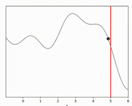
I created a simple physics simulation where the objective is to push a particle to a target location over a hilly 1-d curve. Its essentially a mountain car problem, but with customised landscapes. In addition, I’ve given the particle fuel - which is finite and contributes to its mass. The reward function for this environment is:
\[R_{t} = -((p_{t} - \tau)^2 + u_{t}^2)\]Where $p_{t}$ is the position of the particle on the x-axis, $\tau$ is the target location on the x-axis and $u_{t}$ is the action input. This is different from the typical mountain-cart environment which has a sparse reward (+1 for reaching goal, $u_{t}^2$ otherwise). Note that $u_{t} \in [0,1]$ which we achieve by applying tanh squashing to a real-valued input.
There is also a ‘terminal’ reward given by:
\[\phi = R_{T} + v_{T}^2\]Which adds the square of the final velocity ($v_{T}$) to each trajectory. This is important as it can stablise some algorithms (particularly GB-MPC) as they optimise the reward for the rolled-out trajectory, but don’t consider any future rewards outside of this trajectory. My approach is a bit hacky as technically the terminal reward should represent the reward over an infinite trajectory (i.e. what the value function does in RL), but to do this correctly, you need to factor in the environment dynamics to figure out a steady state. I didnt do this because firstly, I wasn’t quite sure how to do this and, secondly, I wanted to treat the environment as a black-box as much as possible.
The results
I ran each of the algorithms five times (to account for randomness in the action sampling) on a single landscape. Each algorithm has access to the exact dynamics of the environment - so they will know exactly what happens for any given action. This enables us to focus on the impact of the algorithms themselves.
I’ve used the below landscape. I like this landscape because the target location (the vertical red line) is on a slope, requiring the algorithm to maintain position while working against gravity.
The results below show that all algorithms are able to achieve a reward close to 0 within 100 timesteps. Admittedly, it is a relatively simple environment, and the algorithms do have perfect knowledge on what is going to happen via their dynamics model. However, it is clear that Random Shooting has (unsurprisingly) much more varied results. GB-MPC also has a bit more variance, perhaps due to the susceptibility of gradient descent to fall into local minima or due to the heuristic nature of the terminal reward.
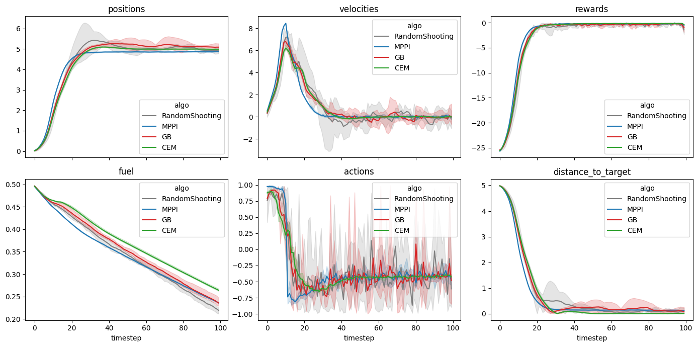
MPPI and CEM are much more stable, with MPPI making the fastest initial progress while CEM eventually achieves a result closer to the target. I’m not completely sure why this is. Looking at some random runs below we see the MPPI sits just above the target line, while the CEM finds the exact point. I speculate that this might be because the MPPI algorithm retains randomness in its action selection process while the CEM updates the standard deviation to get narrower distributions. In complex environments this could actually be a drawback, but here it may have been beneficial.
Conclusion and reflections
So I hope that now you have a reasonable understanding of the above MPC algorithms. Each of these algorithms can be applied to a simulation environment if you have a model of the dynamics and a reward function. In addition, if you don’t know the environment dynamics you could learn them and apply these algorithms on top of your learnt dynamics model. But they key point I want to emphasise, is that these algorithms can be implemented simply without knowledge of the environment dynamics or how rewards are measured because these are simply inputs that are provided.
Here is a brief summary of (some of) the pros and cons of each method:
| Algorithm | Pros | Cons |
|---|---|---|
| Random Shooting | • Simple to implement • Works with any model (non-differentiable) |
• Sample inefficient (esp in high dimensions) • No “intelligence” in search |
| CEM (Cross-Entropy) | • Searches intelligently and improves actions • Works with any model (non-differentiable) |
• Can collapse to a single point too early by updating standard deviation • Sensitive to the “Elite” count hyperparameter |
| MPPI | • Maintains a probability distribution over actions • Works with any model (non-differentiable) • Probabilistic foundations help it to explore |
• May need to tune hyper-parameters (Temperature $\lambda$ and $\Sigma$) |
| GB-MPC (Gradient-Based) | • Most efficient for high-dimensional actions |
• Requires a differentiable model ($f_\theta$) • Prone to getting stuck in local optima • Vanishing/Exploding gradients over long horizons |
Before concluding, its worth reflecting that these MPC algorithms were able to solve the above environments in a single episode and within a few timesteps. Of course, this example was pretty simple and there are a number of elements worth exploring further.
Firstly, we gave all of the algorithms access to the true dynamics model. In many circumstances we would need to learn the model, and I expect this would take several episodes. This is a topic I’d like to explore in more detail in a future article.
Secondly, our reward provided an unambiguous representation of our goal (reach $x=5$). The typical Mountain Car environment does not specify the reward location and gives a sparse reward. This would make the application of MPC harder even if you had access to the true dynamics model. You may need to encourage exploration or use a larger rollout length to enable the agent to discover the reward. Failure to do this can lead to agents sitting still where the action penalty $u_{t}^2 = 0$.
Thirdly, I haven’t actually compared any of these MPC approaches against an RL agent. I should do this to see if using MPC is faster. My gut feel is that an RL agent would require at least a few episodes to learn a simple environment like this. My initial go-to algorithm for a simple environment like this would be temporal differencing as it can learn online. What I am really keen to understand though, is whether learning a dynamics model and optimising using MPC is genuinely faster than a model free approach. I believe this is widely considered to be true, but I’m not entirely sure I understand why - I would have thought learning a dynamics model is pretty hard!
Anyway, for those of you that made it to the end I hope this has been an interesting read. Thanks for reading!
References
-
Botev, Z. I., Kroese, D. P., Rubinstein, R. Y., & L’Ecuyer, P. (2013). The Cross-Entropy Method for Optimization. Handbook of Statistics, 31, 35-59. ↩ ↩2
-
Bharadhwaj, H., Xie, K., & Shkurti, F. (2020). Model-Predictive Control via Cross-Entropy and Gradient-Based Optimization. Proceedings of the 2nd Conference on Learning for Dynamics and Control, PMLR 120:277-286. ↩ ↩2
-
Williams, G., Wagener, N., Goldfain, B., Drews, P., Rehg, J. M., Boots, B., & Theodorou, E. A. (2017). Information Theoretic MPC for Model-Based Reinforcement Learning. IEEE International Conference on Robotics and Automation (ICRA), 1714-1721. ↩ ↩2
-
Williams, G., Drews, P., Goldfain, B., Rehg, J. M., & Theodorou, E. A. (2018). Information-Theoretic Model Predictive Control: Theory and Applications to Autonomous Driving. IEEE Transactions on Robotics, 34(6), 1603-1622. ↩
-
Honda, K. (2025). Model Predictive Control via Probabilistic Inference: A Tutorial. arXiv, arXiv.org/abs/2511.08019 ↩